Using MACSio
MACSio is probably very different from many other I/O benchmarking tools you
may be familiar with. To orient yourself, it may be useful to read the first
sections of the original design document.
In particular, in MACSio_ speak, when we talk about I/O requests, request sizes, frequencies, etc., we speak about them in terms of the operations of a real application performing dumps of its mesh and field data.
By default, MACSio’s command-line arguments are designed to maintain constant per-task I/O workload as task count is varied. This means MACSio, by default, exhibits weak scaling behavior. This does not mean, however, that strong scaling scenarios cannot also be handled. It means only that extra work is involved in constructing command-line arguments to ensure a strong scaling goal is achieved if that is desired.
MACSio has a large number of command-line arguments. In addition, each plugin may define additional command-line arguments. Full documentation of all MACSio’s command-line arguments and their meaning can be obtained with the command
% ./macsio --help | more
Be ready for a lot of output!
Here, we will describe only some of the basic arguments necessary to do initial testing that MACSio is installed correctly and to scale to large sizes.
All command-line arguments specified after the keyword argument --plugin_args
are passed to the plugin and not interpreted by MACSio’s main.
Summary of Key Command Line Arguments
MACSio has many command-line arguments and that number is only likely to grow with time. We discuss here, only those the most relevant to initially getting started running MACSio tests.
MACSio is different from I/O benchmarking tools because it constructs and marshals data as real data objects commonly used in scientific computing applications. All of its command-line arguments are designed in these terms and one has to understand how those choices effect I/O workload created by MACSio.
In the descriptions below, default values for all command-line arguments are indicated in square brackets.
- –interface
--interface %s [miftmpl] Specify the name of the interface (e.g. plugin) to be tested. Use keyword list to print a list of all known interface names and then exit. Examples:
Get list of available plugins
% ./macsio --interface list
List of available I/O-library plugins...
"miftmpl", "hdf5", "silo", "typhonio"
Use the HDF5 plugin for a given test
% ./macsio --interface hdf5
- –parallel_file_mode
--parallel_file_mode %s %d [MIF 4] Specify the parallel file mode. There are several choices. Not all parallel modes are supported by all plugins. Use ‘MIF’ for Multiple Independent File (MIF) mode and then also specify the number of files. Or, use ‘MIFFPP’ for MIF mode and one file per task and where macsio uses known task count. Use ‘MIFOPT’ for MIF mode and let MACSio determine an optimum file count based on heuristics. Use ‘SIF’ for SIngle shared File mode. If you also give a file count for SIF mode, then MACSio will perform a sort of hybrid combination of MIF and SIF modes. It will produce the specified number of files by grouping tasks in the the same way MIF does, but I/O within each group will be to a single, shared file using SIF mode and a subsetted communicator. When using SIF parallel mode, be sure you are running on a true parallel file system (e.g. GPFS or Lustre).
- –part_type
--part_type %s [rectilinear] Options are ‘uniform’, ‘rectilinear’, ‘curvilinear’, ‘unstructured’ and ‘arbitrary’. Generally, this option impacts only the I/O worload associated with the mesh object itself and not any variables defined on the mesh. However, not all I/O libraries (or their associated MACSio plugins) support all mesh types and when making comparisons it is important to have the option of specifying various mesh types.
- –part-dim
--part_dim %d [2] Spatial dimension of mesh parts; 1, 2, or 3. In most cases, 2 is a good choice because it makes downstream visualization of MACSio data easier and more natural. While MACSio is designed such that we would not ordinarily expect I/O workload to be substantially different for different spatial dimensions, this isn’t always known to be true for all possible plugins ahead of time.
- –part_size
--part_size %d [80000] Per-task mesh part size. This becomes the nominal I/O request size used by each task when marshaling data. A following
B|K|M|Gcharacter indicates ‘B’ytes, ‘K’ilo-, ‘M’ega- or ‘G’iga- bytes representing powers of either 1000 or 1024 depending on the selected units prefix system. With no size modifier character, ‘B’ytes is assumed. Mesh and variable data is then sized by MACSio to hit this target byte count in I/O requests. However, due to constraints involved in creating valid mesh topology and variable data with realistic variation in features (e.g. zone- and node-centering), this target byte count is hit exactly for only the most commonly used objects and approximately for other objects.- –avg_num_parts
--avg_num_parts %f [1] The average number of mesh parts per task. Non-integral values are acceptable. For example, a value that is half-way between two integers, K and K+1, means that half the task have K mesh parts and half have K+1 mesh parts, a typical scanrio for multi-physics applications. As another example, a value of 2.75 here would mean that 75% of the tasks get 3 parts and 25% of the tasks get 2 parts. Note that the total number of parts is this number multiplied by the task count. If the result of that product is non-integral, it will be rounded and a warning message will be generated.
- –vars_per_part
--vars_per_part %d [20] Number of mesh variables on each part. This controls the number of I/O requests each task makes to complete a given dump. Typical physics simulations run with anywhere from just a few effectively to several hundred mesh variables. Note that the choice in mesh part_type sets a lower bound on the effective number of mesh variables marshaled by MACSio due to the storage involved for the mesh coordinate and topology data alone. For example, for a uniform mesh this lower bound is effectively zero because there is no coordinate or topology data for the mesh itself. This is also almost true for rectilinear meshes. For curvilinear mesh the lower bound is the number of spatial dimensions and for unstructured mesh it is the number of spatial dimensions plus 2^number of topological dimensions.
Note
uniform vs. rectilinear not fully defined here.
- –num_dumps
--num_dumps %d [10] Total number of dumps to marshal
- –dataset_growth
--dataset_growth %f [1] A multiplier factor by which the volume of data will grow between dump iterations If no value is given or the value is <1.0 no dataset changes will take place.
- –meta_type
--meta_type %s [tabular] Specify the type of metadata objects to include in each main dump. Options are ‘tabular’ or ‘amorphous’. For tabular type data, MACSio will generate a random set of tables of somewhat random structure and content. For amorphous, MACSio will generate a random hierarchy of random type and sized objects.
- –meta_size
--meta_size %d %d [10000 50000] Specify the size of the metadata objects on each task and separately, the root (or master) task (MPI rank 0). The size is specified in terms of the total number of bytes in the metadata objects MACSio creates. For example, a type of tabular and a size of 10K bytes might result in 3 random tables; one table with 250 unnamed records where each record is an array of 3 doubles for a total of 6000 bytes, another table of 200 records where each record is a named integer value where each name is length 8 chars for a total of 2400 bytes and a 3rd table of 40 unnamed records where each record is a 40 byte struct comprised of ints and doubles for a total of 1600 bytes.
- –compute_work_intensity
--compute_work_intensity %d [0] Add some compute workload (e.g. give the tasks something to do) between I/O dumps. There are three levels of ‘compute’ that can be performed as follows:
Level 1: Perform a basic sleep operation (this is the default)
Level 2: Perform some simple FLOPS with randomly accessed data
Level 3: Solves the 2D Poisson equation via the Jacobi iterative method
This input is intended to be used in conjunection with –compute_time which will roughly control how much time is spent doing work between dumps.
- –time_randomize
--time_randomize [0] Make randomization in MACSio vary from dump to dump within a given run and from run to run by using PRNGs seeded by time.
- –plugin-args
--plugin_args All arguments after this sentinel are passed to the I/O plugin plugin.
MACSio Command Line Examples
To run with Multiple Independent File (MIF) mode to on 93 tasks to 8 HDF5 files…
mpirun -np 93 macsio --interface hdf5 --parallel_file_mode MIF 8
Same as above to but a Single Shared File (SIF) mode to 1 HDF5 file (note: this is possible with the same plugin because the HDF5 plugin in MACSio has been designed to support both the MIF and SIF parallel I/O modes.
mpirun -np 93 macsio --interface hdf5 --parallel_file_mode SIF 1
Default per-task request size is 80,000 bytes (10K doubles). To use a different request size, use –part_size. For example, to run on 128 tasks, 8 files in MIF mode where I/O request size is 10 megabytes, use
mpirun -np 128 macsio --interface hdf5 --parallel_file_mode MIF_ 8 --part_size 10M
Here, the
Mafter the10means either decimal Megabytes (Mb) or binary Mibibytes (Mi) depending on setting for--units_prefix_system. Default is binary.To use H5Z-ZFP compression plugin (note: we’re talking about an HDF5 plugin here), be sure to have the plugin compiled and available with the same compiler and version of HDF5 you are using with MACSio. Here, we demonstrate a MACSio command line that runs on 4 tasks, does MIF parallel I/O mode to 2 files, on a two dimensional, rectilinear mesh with an average number of parts per task of 2.5 and a nominal I/O request size of 40,000 bytes. The args after
--plugin-argsare to specify ZFP compression parameters to the HDF5 plugin. In this case, we use H5Z-ZFP compression plugin in rate mode with a bit-rate of 4.env HDF5_PLUGIN_PATH=<path-to-plugin-dir> mpirun -np 4 ./macsio --interface hdf5 --parallel_file_mode MIF 2 --avg_num_parts 2.5 --part_size 40000 --part_dim 2 --part_type rectilinear --num_dumps 2 --plugin_args --compression zfp rate=4
where
path-to-plugin-diris the path to the directory containinglibh5zzfp.{a,so,dylib}
Weak Scaling Study Command-Line Example
Suppose you want to perform a weak scaling study with MACSio in MIF parllel I/O mode and where per-task I/O requests are nominally 100 kilobytes and each task has 8 mesh parts.
All MACSio command line arguments remain the same. The only difference is the task count you execute MACSio with.
for n in 32 64 128 256 512 1024 2048 4096
do
    mpirun -np $n macsio --interface hdf5 --avg_num_parts 8 --part_size 100K --parallel_file_mode MIF 32
done
Now, the above example started with a task count of 32 and 32 files in MIF mode and kept the file count constant. It is concievable that if you continued this study to larger and larger scales, you may also want the MIF file count to vary somewhat as well. Here is an example of doing that.
Example
Which when run, results in the following sequence of MACSio command-lines.
mpirun -np 32 macsio --interface hdf5 --avg_num_parts 8 --part_size 100K --parallel_file_mode MIF 32
mpirun -np 64 macsio --interface hdf5 --avg_num_parts 8 --part_size 100K --parallel_file_mode MIF 64
mpirun -np 128 macsio --interface hdf5 --avg_num_parts 8 --part_size 100K --parallel_file_mode MIF 64
mpirun -np 256 macsio --interface hdf5 --avg_num_parts 8 --part_size 100K --parallel_file_mode MIF 64
mpirun -np 512 macsio --interface hdf5 --avg_num_parts 8 --part_size 100K --parallel_file_mode MIF 64
mpirun -np 1024 macsio --interface hdf5 --avg_num_parts 8 --part_size 100K --parallel_file_mode MIF 64
mpirun -np 2048 macsio --interface hdf5 --avg_num_parts 8 --part_size 100K --parallel_file_mode MIF 64
mpirun -np 4096 macsio --interface hdf5 --avg_num_parts 8 --part_size 100K --parallel_file_mode MIF 64
mpirun -np 8192 macsio --interface hdf5 --avg_num_parts 8 --part_size 100K --parallel_file_mode MIF 64
mpirun -np 16384 macsio --interface hdf5 --avg_num_parts 8 --part_size 100K --parallel_file_mode MIF 128
mpirun -np 32768 macsio --interface hdf5 --avg_num_parts 8 --part_size 100K --parallel_file_mode MIF 128
mpirun -np 65536 macsio --interface hdf5 --avg_num_parts 8 --part_size 100K --parallel_file_mode MIF 128
mpirun -np 131072 macsio --interface hdf5 --avg_num_parts 8 --part_size 100K --parallel_file_mode MIF 256
mpirun -np 262144 macsio --interface hdf5 --avg_num_parts 8 --part_size 100K --parallel_file_mode MIF 256
Because the default mesh type is rectilinear (which involves very little in the way of I/O for the mesh itself),
the default number of mesh variables is 20, for a typical plugin running the MIF parallel I/O mode,
each task will emit 8*20 (there are 8 mesh parts per task), 100K writes for a given dump. The default number of
dumps is 10, so this will be repeated 10 times. For a --parallel_file_mode MIF 32 run, each dump will produce
32 files for a total of 320 files produced for that first run. In the first run, because file count and
task count are 1:1, each file will contain just 8 mesh parts. For the last run, there are 256 files per dump
but 262144 tasks, each task having 8 mesh parts. So, each file would, in that case, contain 8192 mesh parts.
Now, because the HDF5 plugin also supports the SIF parallel I/O mode, we could run the same sequence of tests
in that mode by replacing MIF XX with SIF.
Strong Scaling Study Command-Line Example
Suppose we wish to perform a strong scaling study. In this case, we need to settle upon the global final mesh size and then construct MACSio command lines for each run such that the task count together with the per-task command-line arguments results in the same (or approximately so) global final mesh object in each run.
In the preceding weak scaling example, MACSio generated a global mesh of size in the range [8*32*100K, 8*262144*100K]. Selecting a middle-of-the-range run of 8*8192*100K (6,710,886,400 bytes) as a nominal global mesh size, we can then use a given task count to determine part size and average part count to hit that target global size. We demonstrate this in the following code block…
When this shell code is run, it results in the following sequence of MACSio command-lines. Note that we cap the total number of files at 1024. Depending on the particular system where this is run, this cap may be too low or too high. The best number is the number of I/O nodes a given instance of MACSio can see when running. Because this number typically varies with task count and where on the system the tasks are actually allocated, this number is not always easily known or obtained.
mpirun -np 32 ./macsio --interface hdf5 --avg_num_parts 2048 --part_size 102400 --parallel_file_mode MIF 32
mpirun -np 64 ./macsio --interface hdf5 --avg_num_parts 1024 --part_size 102400 --parallel_file_mode MIF 64
mpirun -np 128 ./macsio --interface hdf5 --avg_num_parts 512 --part_size 102400 --parallel_file_mode MIF 128
mpirun -np 256 ./macsio --interface hdf5 --avg_num_parts 256 --part_size 102400 --parallel_file_mode MIF 256
mpirun -np 512 ./macsio --interface hdf5 --avg_num_parts 128 --part_size 102400 --parallel_file_mode MIF 512
mpirun -np 1024 ./macsio --interface hdf5 --avg_num_parts 64 --part_size 102400 --parallel_file_mode MIF 1024
mpirun -np 2048 ./macsio --interface hdf5 --avg_num_parts 32 --part_size 102400 --parallel_file_mode MIF 1024
mpirun -np 4096 ./macsio --interface hdf5 --avg_num_parts 16 --part_size 102400 --parallel_file_mode MIF 1024
mpirun -np 8192 ./macsio --interface hdf5 --avg_num_parts 8 --part_size 102400 --parallel_file_mode MIF 1024
mpirun -np 16384 ./macsio --interface hdf5 --avg_num_parts 4 --part_size 102400 --parallel_file_mode MIF 1024
mpirun -np 32768 ./macsio --interface hdf5 --avg_num_parts 2 --part_size 102400 --parallel_file_mode MIF 1024
mpirun -np 65536 ./macsio --interface hdf5 --avg_num_parts 1 --part_size 102400 --parallel_file_mode MIF 1024
mpirun -np 131072 ./macsio --interface hdf5 --avg_num_parts 1 --part_size 51200 --parallel_file_mode MIF 1024
mpirun -np 262144 ./macsio --interface hdf5 --avg_num_parts 1 --part_size 25600 --parallel_file_mode MIF 1024
To perform a strong scaling study in SIF parallel I/O mode, just replace the trailing
MIF $nf in the above MACSio command line above with SIF.
This strong scaling scenario maintains constant part size (up to the last three iterations) and just varies the part count to hit the target global size. Instead, we may want to do a strong scaling scenario where we maintain just a single part per task and vary that single part’s size to hit the target global size. This is demonstrated with following code…
which prodcues the following sequence of MACSio command-lines…
mpirun -np 32 ./macsio --interface hdf5 --avg_num_parts 1 --part_size 209715200 --parallel_file_mode MIF 32
mpirun -np 64 ./macsio --interface hdf5 --avg_num_parts 1 --part_size 104857600 --parallel_file_mode MIF 64
mpirun -np 128 ./macsio --interface hdf5 --avg_num_parts 1 --part_size 52428800 --parallel_file_mode MIF 128
mpirun -np 256 ./macsio --interface hdf5 --avg_num_parts 1 --part_size 26214400 --parallel_file_mode MIF 256
mpirun -np 512 ./macsio --interface hdf5 --avg_num_parts 1 --part_size 13107200 --parallel_file_mode MIF 512
mpirun -np 1024 ./macsio --interface hdf5 --avg_num_parts 1 --part_size 6553600 --parallel_file_mode MIF 1024
mpirun -np 2048 ./macsio --interface hdf5 --avg_num_parts 1 --part_size 3276800 --parallel_file_mode MIF 1024
mpirun -np 4096 ./macsio --interface hdf5 --avg_num_parts 1 --part_size 1638400 --parallel_file_mode MIF 1024
mpirun -np 8192 ./macsio --interface hdf5 --avg_num_parts 1 --part_size 819200 --parallel_file_mode MIF 1024
mpirun -np 16384 ./macsio --interface hdf5 --avg_num_parts 1 --part_size 409600 --parallel_file_mode MIF 1024
mpirun -np 32768 ./macsio --interface hdf5 --avg_num_parts 1 --part_size 204800 --parallel_file_mode MIF 1024
mpirun -np 65536 ./macsio --interface hdf5 --avg_num_parts 1 --part_size 102400 --parallel_file_mode MIF 1024
mpirun -np 131072 ./macsio --interface hdf5 --avg_num_parts 1 --part_size 51200 --parallel_file_mode MIF 1024
mpirun -np 262144 ./macsio --interface hdf5 --avg_num_parts 1 --part_size 25600 --parallel_file_mode MIF 1024
The difference in these two strong scaling scenarious is that the first one will suffer from per-part overheads. Each task will have per-part memory overheads and per-part I/O request overheads which the second scenario does not suffer.
Assessing Performance Achieved by MACSio
On the one hand, MACSio tries to boil all the performance data down to a single, scalar
metric; the average time to complete a dump or the average bandwidth for completing
a dump. This information is captured in task 0’s section (header) MACSio’s main log file,
macsio-log.log.
An example is shown below for 10 dumps from a 4 task run.
The key line in the file, for task 0, is the total bytes divided by the time between the last task to finish and the first task to start which looks similar to the line below…
Info:"macsio_main.c":727:Total Bytes: 57.4580 Mi; Last finisher - First starter = 1.5012 secs; BW = 38.2758 Mi/sec:::
Detailed Performance Data
Detailed performance data is captured by MACSio as timers and then
dumped to strings (see MACSIO_TIMING_DumpTimersToStrings() for specific format of dumped
timer data strings) for output to a log file upon exit.
The performance data gathered by MACSio is wholly dependent on the degree to which developers of MACSio or its plugins have instrumented MACSio with suitable timing calls. If timing information provided is not sufficient, the solution is to submit a PR with relevant timer calls added.
Each task maintains its own unique set of timers for its own activities. In addition,
MACSio will reduce all the task-specific timers just prior to completion. All timer data,
the task-specific timers together with the reduced timers, is then dumped to a MACSio log
file with the name macsio-timings.log. That single file captures all of the performance
data for a given run of MACSio.
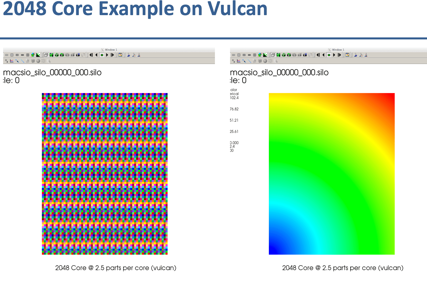
Validating Data MACSio Produces
Most MACSio plugins produce valid scientific computing data which can be processed by other common workflow tools and, in particular, visualization tools such as VisIt, ParaView or Ensight.
The images here demonstrate MACSio, 2D data written with the Silo plugin
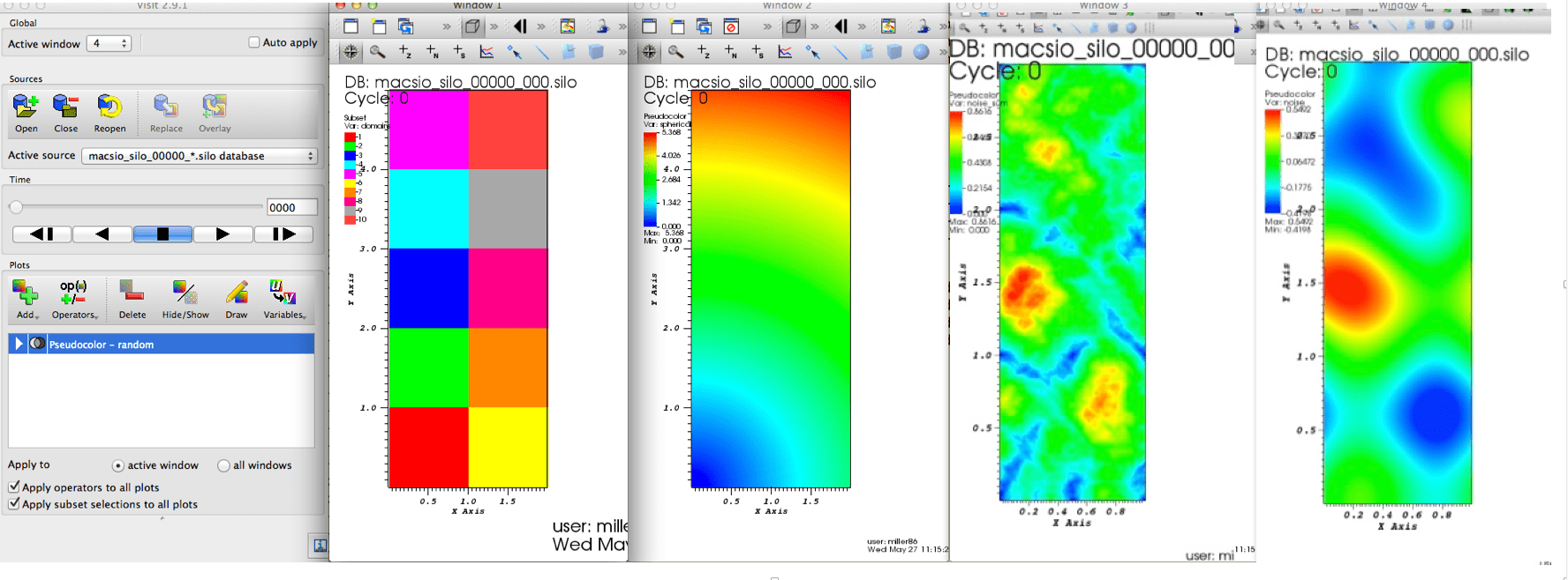
VisIt displaying MACSio produced data on 4 tasks and 2.5 parts per task with the Silo plugin. From left to right, the visualizations display the parallel decomposition of the mesh into blocks, a smoothly varying, node-centered variable on the mesh, a high noise node-centered variable and a low-noise node-centered variable.